Benchmark methodology

Each benchmark is a specific test case for a given simulator that runs on a large number of different hardware resources. The goal is to provide a comprehensive comparison of the performance of different hardware resources for that test case while providing insights into the scalability and efficiency enhancements offered by cloud-based computing solutions for computational needs. Multiple metrics are made available, being the most common the time taken to complete the simulation and the cost of running that simulation. As the project evolves, more metrics will be added to the benchmarks.

The type of resources used in each benchmark session depends on the simulator and, particularly, on how the simulator was compiled. For some simulators, AMD-based builds are not yet available. Again, as the project evolves, these limitations will be removed.

Benchmark outputs

Each benchmark session is directly translated to an independent report that belongs to a specific simulator. Each simulator provides an overview of the simulator itself and lists the benchmarks available for it. Each report is composed of a description of the test case followed by a minimum of two plots, as detailed below. The raw information used to build those plots is available inside collapsible sections; the version and compilation details of the simulator are also provided.

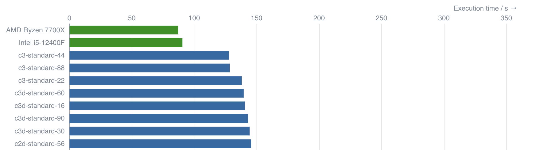
Plot 1 - Execution times

The first plot shows a direct comparison of the average execution times of the test case among the different machine types. The execution times are presented as horizontal bars, sorted in ascending execution order, with shorter bars indicating faster execution times. The cloud machines are colored in blue, while the local baseline machines are, typically, colored green.

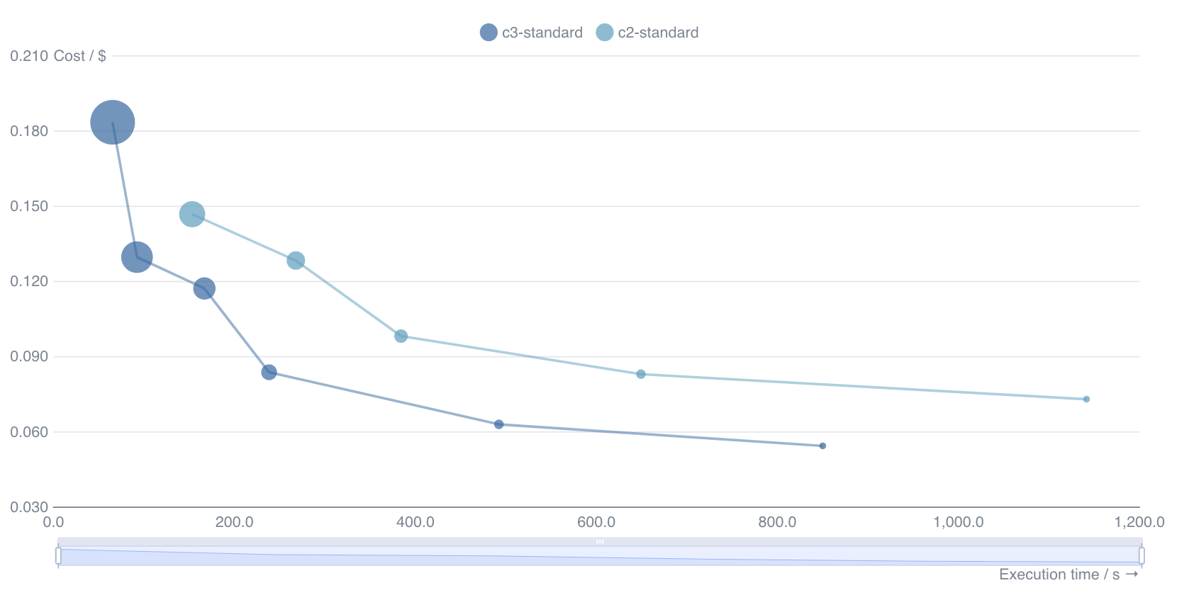
Plot 2 - Simulation Cost vs Execution times

The second plot shows how the run times (x-axis) and simulation costs (y-axis) vary with the number of cores for each machine type, with the number of virtual CPUs encoded in the size of the markers. Generally speaking, the best value for money is found in the bottom left corner of the plot, thus representing the cheapest option that still provides results in a reasonable amount of time.

Statistics

All metrics are calculated using the average of 5 independent runs. When possible, standard deviations are presented alongside the nominal value. Execution times are taken as the wall-clock times, i.e., the time taken to execute the simulation command. The cost of running the simulation is obtained by multiplying the execution time by the price per hour of the target machine.

FAQ

How did we run the benchmark cases locally?

The local runs are executed by deploying the relevant docker container for the simulator on the local machine. The docker containers are available via Kutu, our public image repository, and are the same that run on the GCP cloud using our API. The test case input files are then run manually through the command line. The execution time of the test case is taken as the wall-clock time for the simulation command, just as in the cloud runs. The following snippet exemplifies how we run a test case in a local machine, using the demo files provided by the Inductiva API for the SWAN simulator, and how we use the time command to measure the execution time (2.24 s) of this test case:

	

		
					
		
		
$ wget https://storage.googleapis.com/inductiva-api-demo-files/swan-input-example.zip
$ unzip swan-input-example.zip
$ mv swan-input-example/a11refr.swn swan-input-example/INPUT
$ docker run -it \
    -v ./swan-input-example:/home/swan_test_case \
    inductiva/kutu:swan_v41.45 \
    /bin/bash -c "cd /home/swan_test_case; \
                  time mpirun --allow-run-as-root --use-hwthread-cpus -np 1 swan.exe"

SWAN is preparing computation

 iteration    1; sweep 1
[...truncated output...]
+SWAN is processing output request    4

real    0m2.240s    # <--- This is the wall-clock time used to run the simulation
user    0m2.132s
sys     0m0.064s
		

How do local runs differ from the ones executed using the API over Google Compute Platform (GCP)?

The local test cases are executed inside a containerized environment using Docker, which runs directly on top of the kernel. This resembles a typical local installation in which Docker is installed on the OS that runs directly on "bare metal". No additional layers of virtualization are present in this setup. However, the test cases executed using the API on the Google Compute Platform run inside a container that runs on top of a virtual machine that runs on top of the Google Cloud infrastructure. This means that there are additional layers of virtualization between the test case and the physical hardware. This difference can have an impact on the run times of the test cases, which are not trivial to quantify. Also, the simulations running through the API use Apptainer containers which are more suitable for HPC workloads, which might also impact the execution times. As the project evolves, we will provide more detailed information on the differences between the local and cloud runs, and attempt to quantify the impact of the additional layers of virtualization on the run times.